Take-home Exercise 3

Published

June 18, 2023

VAST Challenge: Mini-Challenge 3

Project Brief

FishEye International, a non-profit focused on countering illegal, unreported, and unregulated (IUU) fishing, has been given access to an international finance corporation’s database on fishing related companies. In the past, FishEye has determined that companies with anomalous structures are far more likely to be involved in IUU (or other fishy business). FishEye has transformed the database into a knowledge graph, including information about companies, owners, workers, and financial status. FishEye is aiming to use this graph to identify anomalies that could indicate if a company is involved in IUU.

Project Objectives

This study aims to use visual analytics to understand patterns of groups in the knowledge graph. This will endeavour to:

develop a visual analytics process to find similar companies and group them
focus on presenting key features of the business to the user

This will be done through investigating the following variables:

%%{
  init: {
    "theme": "base",
    "themeVariables": {
      "primaryColor": "#d8e8e6",
      "primaryTextColor": "#325985",
      "primaryBorderColor": "#325985",
      "lineColor": "#325985",
      "secondaryColor": "#cedded",
      "tertiaryColor": "#fff" 
      }
  }
}%%

flowchart LR
    A{Overall\nNetwork} --> B{Companies}
    B -->|Similarities?| C(Company Structure)
    B -->|Similarities?| D(Location)
    B -->|Similarities?| E(Business Type)
    B -->|Similarities?| F(Financial Status)

1: Data Preparation

1.1: Loading R Packages

code block

pacman::p_load(jsonlite, tidyverse, DT, lubridate, Hmisc, 
               urbnthemes,visNetwork, tidygraph, ggraph, 
               ggiraph, igraph, scales, ggplot2, 
               gganimate, ggstatsplot, ggrain, ggridges, 
               graphlayouts, plotly, patchwork, kableExtra, 
               ggpubr, ggrepel, ggforce, tidytext,
               tm, wordcloud2, forcats, skimr, kableExtra)

1.2: Loading the Data

Use jsonlite package to read .json files

mc3 <- fromJSON("data/MC3.json")

mc3 data consists of undirected graph data, with links and nodes. These are stored as lists instead of vector columns. To transform this into a dataframe, each column is mutated into a character data type using mutate() and as.character() methods.

code block

mc3_links <- as_tibble(mc3$links) %>%
  distinct() %>%
  # Change all variable types to character to create dataframe
  mutate(source = as.character(source),
         target = as.character(target),
         type = as.character(type)) %>%
  group_by(source, target, type) %>%
  summarise(weights = n()) %>%
  filter(source != target) %>%
  select(-weights) %>%
  ungroup

mc3_nodes <- as_tibble(mc3$nodes) %>%
  mutate(id = as.character(id), 
         type = as.character(type), 
         country = as.character(country), 
         product_services = as.character(product_services),
  # Convert to character first to unlist, then revert to numeric form 
         revenue_omu = as.numeric(as.character(revenue_omu))) %>%
  # Reorganize columns 
  select(id, country, type, revenue_omu, product_services)

I. Checking for Missing Values:

# Check for columns with missing values
colSums(is.na(mc3_nodes))

              id          country             type      revenue_omu 
               0                0                0            21515 
product_services 
               0

There are 21,515 missing values from the revenue_omu column.

II. Checking for Duplicates

mc3_nodes[duplicated(mc3_nodes),]

# A tibble: 2,595 × 5
   id                              country type    revenue_omu product_services
   <chr>                           <chr>   <chr>         <dbl> <chr>           
 1 Smith Ltd                       ZH      Company          NA Unknown         
 2 Williams LLC                    ZH      Company          NA Unknown         
 3 Garcia Inc                      ZH      Company          NA Unknown         
 4 Walker and Sons                 ZH      Company          NA Unknown         
 5 Walker and Sons                 ZH      Company          NA Unknown         
 6 Smith LLC                       ZH      Company          NA Unknown         
 7 Smith Ltd                       ZH      Company          NA Unknown         
 8 Romero Inc                      ZH      Company          NA Unknown         
 9 Niger River   Marine life       Oceanus Company          NA Unknown         
10 Coastal Crusaders AS Industrial Oceanus Company          NA Unknown         
# ℹ 2,585 more rows

There are 2,595 duplicated entries. These are removed so as to prevent skewing of aggregate figures in subsequent analyses:

mc3_nodes <- unique(mc3_nodes)

There are several ids from the same country and type, but different revenue and products_services values. These are collapsed so as not to skew the analysis:

mc3_nodes_new <- mc3_nodes %>%
  group_by(id, country, type) %>%
  summarise(revenue_omu = sum(revenue_omu),
            product_services = paste(product_services, collapse = ", "))

I. Checking for Missing Values:

# Check for columns with missing values
colSums(is.na(mc3_links))

source target   type 
     0      0      0

There are no missing values in mc3_links

II. Cleaning up grouped data in Source column

Source column contains vector-like strings with multiple company names, eg. c(“Yu er he Solutions”, “Yu er he Solutions”,). This is extracted and split into separate rows, also duplicating the original values from variables across the columns:

mc3_links_new <- mc3_links %>%
  # Extract all text within " "
  mutate(source = str_extract_all(source, '"(.*?)"')) %>%
  # Split into separate rows
  unnest(source) %>%
  # Split phrases by comma ignoring leading spaces
  separate_rows(source, sep = ",\\s*") %>%
  mutate(source = str_remove_all(source, '"')) %>%
  fill(everything())

III. Checking for Duplicates:

mc3_links_new[duplicated(mc3_links_new),]

# A tibble: 2,238 × 3
   source                      target           type            
   <chr>                       <chr>            <chr>           
 1 1 Ltd. Liability Co         Yesenia Oliver   Company Contacts
 2 1 Swordfish Ltd Solutions   Daniel Reese     Company Contacts
 3 6 GmbH & Co. KG             Monique Cummings Company Contacts
 4 6 GmbH & Co. KG             Monique Cummings Company Contacts
 5 Mar de la Luz BV            Monique Cummings Company Contacts
 6 7 Ltd. Liability Co Express Cassidy Sherman  Beneficial Owner
 7 7 Ltd. Liability Co Express Dawn West        Beneficial Owner
 8 7 Ltd. Liability Co Express Hannah Franco    Company Contacts
 9 7 Ltd. Liability Co Express Michael Morrison Beneficial Owner
10 7 Ltd. Liability Co Express Nicole Carrillo  Beneficial Owner
# ℹ 2,228 more rows

There are 2,238 duplicated rows for mc3_links data. These are removed using the unique() function:

mc3_links_new <- unique(mc3_links_new)

2: Exploratory Analysis

skim(mc3_links_new)

Data summary
Name	mc3_links_new
Number of rows	3064
Number of columns	3
_______________________
Column type frequency:
character	3
________________________
Group variables	None

Variable type: character

skim_variable	complete_rate	min	max	n_unique
source	1	13	56	1160
target	1	7	23	2140
type	1	16	16	2

skim() shows that the links data consists of 1160 unique source and 2140 unique target nodes. To reducing the dimensionality of the data is thus imperative in creating useful network visualisations. Further exploratory analysis needs to be conducted to deduce the filtering criteria for determining anomalous groups.

Who are the Stakeholders?

Nodes data is aggregated by country and type to visualise frequency of roles, as well as where each company or person is operating geographically.

code block

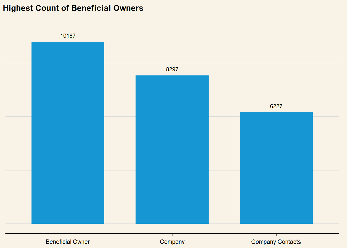
# Set default plot theme
set_urbn_defaults(style = "print")

nodes_type <- mc3_nodes_new %>%
  ggplot(
    aes(x = type)
  ) +
  geom_bar() +
 # Set count annotations above bar
  geom_text(
    stat = "count",
    aes(label = after_stat(count)),
    vjust = -1
  ) +  
 # Ensure than annotations are not cut off
  ylim(0, 11000) +
  labs(
    title = "Highest Count of Beneficial Owners"
  ) +
  theme(
    axis.title.y = element_blank(),
    axis.title.x = element_blank(),
    axis.text.y = element_blank(),
    plot.background = element_rect(fill="#F8F3E6",colour="#F8F3E6")
  )

nodes_type

Where are they operating from?

code block

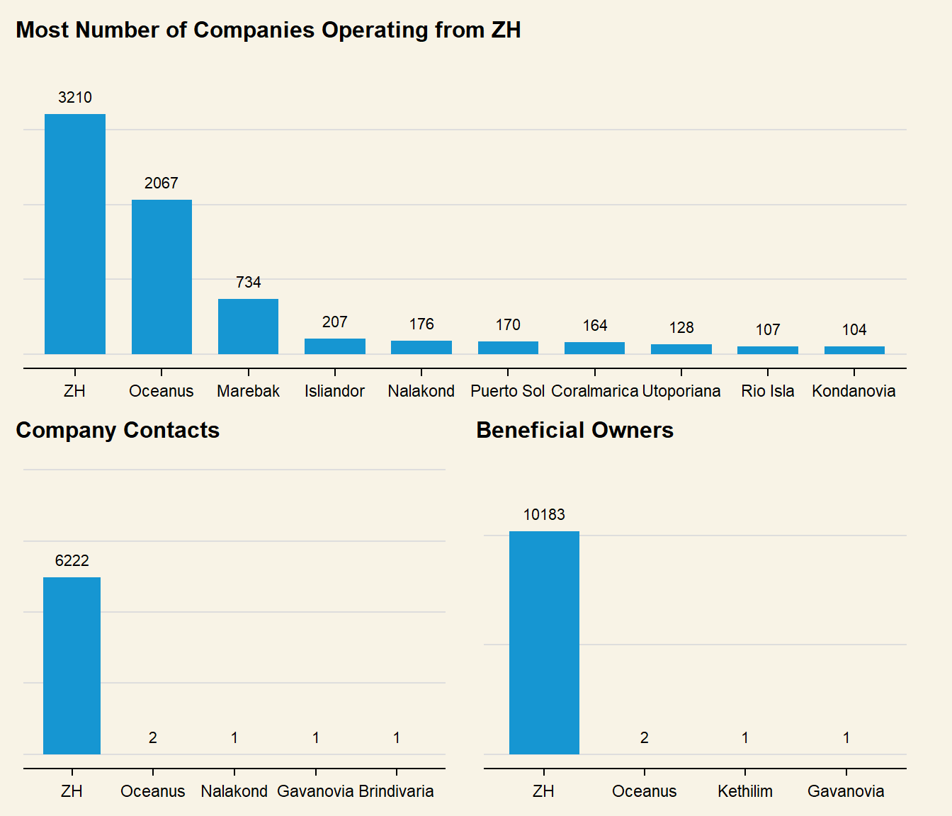
# Aggregate data frame by country and type
nodes_agg <- mc3_nodes_new %>%
  group_by(country, type) %>%
  # Count number of companies per country
  summarise(count = n(),
  # Calculate total revenue per country
            revenue_omu = sum(revenue_omu)) %>%
  ungroup()


# Create separate plots for each type
p_company <- nodes_agg %>%
  # Only plot countries with more than 100 companies
  filter(type == "Company" &
           count > 100) %>%
  ggplot(
  # Arrange in Descending order of count
    aes(x = fct_rev(fct_reorder(country, count)),
        y = count)
  ) +
  geom_col() +
  # Set to prevent trunctation when patched
  ylim(0,3800) +
  geom_text(
    aes(label = count),
    vjust = -1
  ) +  #< Set count annotations above bar
  labs(
    title = "Most Number of Companies Operating from ZH"
  ) +
  theme(
    axis.title.y = element_blank(),
    axis.title.x = element_blank(),
    axis.text.y = element_blank(),
    plot.background = element_rect(fill="#F8F3E6",colour="#F8F3E6")
  )

# Plot for company contacts
p_contact <- nodes_agg %>%
  # Only plot countries with more than 100 companies
  filter(type == "Company Contacts") %>%
  ggplot(
  # Arrange in Descending order of count
    aes(x = fct_rev(fct_reorder(country, count)),
        y = count)
  ) +
  geom_col() +
  geom_text(
    aes(label = count),
    vjust = -1
  ) + 
  ylim(0,10000) +
  labs(
    title = "Company Contacts"
  ) +
  theme(
    axis.title.y = element_blank(),
    axis.title.x = element_blank(),
    axis.text.y = element_blank(),
    plot.background = element_rect(fill="#F8F3E6",colour="#F8F3E6")
  )

# Plot for beneficial owners
p_owner <- nodes_agg %>%
  # Only plot countries with more than 100 companies
  filter(type == "Beneficial Owner") %>%
  ggplot(
  # Arrange in Descending order of count
    aes(x = fct_rev(fct_reorder(country, count)),
        y = count)
  ) +
  geom_col() +
  geom_text(
    aes(label = count),
    vjust = -1
  ) +
  ylim(0,13000) +
  labs(
    title = "Beneficial Owners"
  ) +
  theme(
    axis.title.y = element_blank(),
    axis.title.x = element_blank(),
    axis.text.y = element_blank(),
    plot.background = element_rect(fill="#F8F3E6",colour="#F8F3E6")
  )

bottompatch <- (p_contact + p_owner) +
  plot_annotation(title = "Almost all Company Contacts & Beneficial Owners from ZH")

fullpatch <- p_company / bottompatch
fullpatch & theme(plot.background = element_rect(fill="#F8F3E6",colour="#F8F3E6"))

Who are the companies connected to?

code block

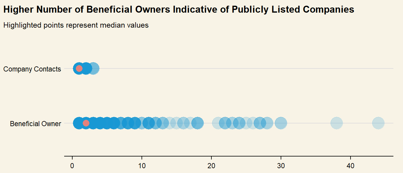
# Get number of type by source (Company)
links_count <- mc3_links_new %>%
  group_by(source, type) %>%
  summarise(count = n()) %>%
  ungroup()

# Plot strip chart to show distibution

links_count %>%
  ggplot(
    aes(x = count, 
        y = type)
  ) +
  geom_point(
    alpha = .2, 
    size = 7
  ) +
  scale_x_continuous() +  
  stat_summary(
    color = "salmon", 
    fun = "median", 
    geom = "point", 
    size = 3.5, 
    alpha = .9
  ) +
  labs(title = "Higher Number of Beneficial Owners Indicative of Publicly Listed Companies",
       subtitle = "Highlighted points represent median values",
       x = NULL,
       y = NULL
  ) +
  theme(axis.ticks.y = element_blank(),
        plot.background = element_rect(fill="#F8F3E6",colour="#F8F3E6")
  )

Initial Insights:

Nodes data seems to list all names of Companies, Beneficial Owners as well as Company Contacts in the Fishing Network. Majority of the companies are based in *ZH and Oceanus, with Company Contacts and Beneficial Owners overwhelmingly from ZH**. This suggests that the businesses are concentrated within a smaller geographical scope.
Links Data has ‘source’ and ‘target’ columns, and seem to denote the relationship of individuals (target) to companies (source), as well as classifying the relationship as type: Company Contact or Beneficial Owner.
Counting the number of individuals per type revealed a much larger variation in Beneficial Owner Count, which could be a good variable to use in classifying the company as Publicly listed (high number of beneficial owners - shareholders) or Sole Proprietorship (Single Beneficial Owner). However, this will also have to be further analysed in tandem with company revenue when grouping similar companies together.

How much revenue is being reported by the Companies?

code block

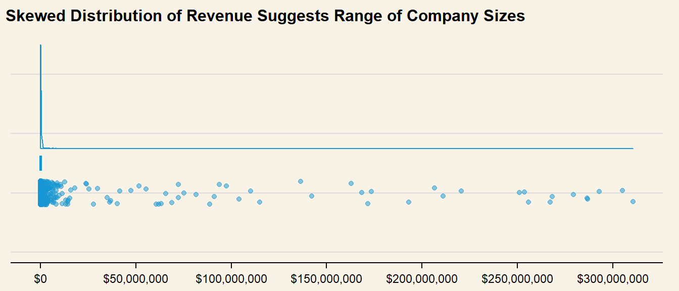
# Only feature data from Companies
company_nodes <- mc3_nodes_new %>%
  filter(type == "Company")

company_rev <-
  ggplot(company_nodes, 
       aes(x = 1, 
           y = revenue_omu)
  ) +
  geom_rain(
    color = "#1696d2",
    alpha = .5
  ) +
  scale_y_continuous(
    breaks = scales::pretty_breaks(n=5),
    labels = scales::dollar
  ) +
  labs(
    title = "Skewed Distribution of Revenue Suggests Range of Company Sizes"
  ) +
  theme(
    axis.ticks.y = element_blank(),
    axis.title = element_blank(),
    axis.text.y = element_blank(),
    plot.background = element_rect(fill="#F8F3E6",colour="#F8F3E6")
  ) +
  coord_flip()

company_rev

Distribution of revenue as well as quantile values show a highly right-skewed distribution, which could be an indication of company size. To use this variable for further classification of anomalous groups, revenue is binned by percentile and assigned a label. As missing Revenue values could be a data lapse issue, or a sign of concealing possible fishy actvity, whis is kept as a separate category for further analysis:

Above 80th Percentile: 1
60-80th Percentile: 2
40-60th Percentile: 3
20-40th Percentile: 4
Below 20th Percentile: 5
Missing Values : NA

code block

# Calculate the percentiles
percentiles <- quantile(mc3_nodes_new$revenue_omu, 
                        probs = c(0, 0.2, 0.4, 0.6, 0.8, 1),
                        na.rm = TRUE)

# Create a new column and assign labels based on percentiles
mc3_nodes_new$revenue_group <- cut(mc3_nodes_new$revenue_omu, 
                                   breaks = percentiles, 
                                   labels = c(5, 4, 3, 2, 1), 
                                   include.lowest = TRUE)

code block

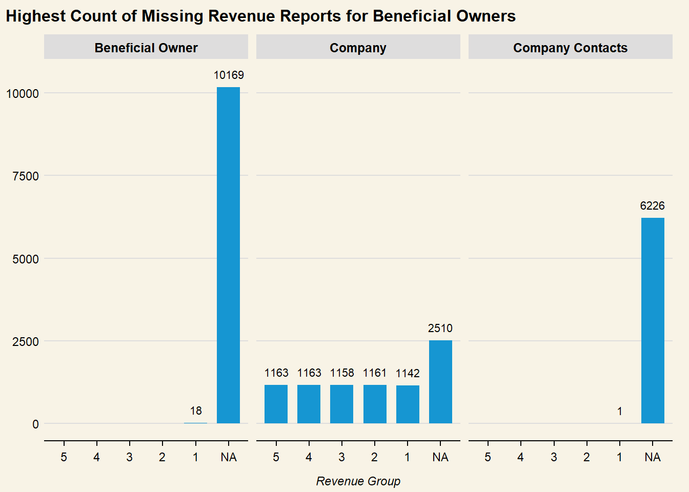
# Barchart of revenue group
ggplot(
  mc3_nodes_new, 
  aes(x = revenue_group)
  ) +
  geom_bar() +
  labs(
    # Linebreak added to title so it does not get truncated
    title = "Highest Count of Missing Revenue Reports for Beneficial Owners", 
    x = "Revenue Group",
    y = NULL
  ) +
  geom_text(
    stat = "count",
    aes(label = after_stat(count)),
    vjust = -1
  ) +
  ylim(0,10500) +
  theme(
    text = element_text(size = 12),
    plot.background = element_rect(fill="#F8F3E6",colour="#F8F3E6")
  ) +
  facet_wrap(~type)

3: Exploring Anomalous Structures

Based on initial analysis, there is an avenue to explore the relationship between different variables to sieve out anomalous groups within the overall network:

%%{
  init: {
    "theme": "base",
    "themeVariables": {
      "primaryColor": "#d8e8e6",
      "primaryTextColor": "#325985",
      "primaryBorderColor": "#325985",
      "lineColor": "#325985",
      "secondaryColor": "#cedded",
      "tertiaryColor": "#fff" 
      }
  }
}%%

flowchart LR
    A{Overall\nNetwork} --> B{Fishy\nCompanies}
    B --> C(Company Structure)
    B --> D(Financial Status) -.->E[High Revenue]
    D -.-> F[Unreported Revenue]
    C -.->|Overlapping?|G[Beneficial Owners]
    C -.->|Overlapping?|H[Company Contacts]

Firstly, the company ownership and company contact structure can be visualised through plotting network graphs. This will give a better sense of how the individual records listed in the links data are related, as well as sieve out possible fishy patterns. The following filters are used to investigate possible ‘groups’ and anomalies:

High Revenue & Companies with Higher numbers of Beneficial Owners
Company Contacts of High Revenue Companies
Unreported Revenue & Higher numbers of Beneficial Owners
Company Contacts of Companies with Unreported Revenue

3.1: What is the structure of companies based on revenue?

3.1.1: High Revenue Groups

Extracting Nodes and Links

# Extract nodes from Highest revenue band
nodes_highrev <- mc3_nodes_new %>%
  filter(revenue_group == "1")

# Only get Beneficial Owners from companies with higher counts
high_owner_count <- links_count %>%
  filter(type == "Beneficial Owner") %>%
  filter(count >20)

links_highrev <- mc3_links_new %>%
  filter(type == "Beneficial Owner") %>%
  filter(source %in% high_owner_count$source) %>%
  filter(source %in% nodes_highrev$id) %>%
  rename("from" = "source",
         "to" = "target")

Getting Distinct Source and Target

# Get distinct Source and Target
hirev_source <- links_highrev %>%
  distinct(from) %>%
  rename("id" = "from")

hirev_target <- links_highrev %>%
  distinct(to) %>%
  rename("id" = "to")

Creating Nodes and Edges Dataframes

# Bind into single dataframe
nodes_hirev_new <- bind_rows(hirev_source, hirev_target)

nodes_hirev_new$group <- ifelse(nodes_hirev_new$id %in% company_nodes$id, "Company", "Beneficial Owner")

code block

visNetwork(
    nodes_hirev_new, 
    links_highrev,
    width = "100%",
    main = list(text = "Fishy Companies with completely overlapping Beneficial Owners:",
                style = "font-size:17x;
                weight:bold;
                text-align:right;"),
    submain = list(text = "Haryana s Catchers ОАО Enterprises & Drakensberg LLC",
                   style = "font-size:13pm; 
                   text-align:right;")
  ) %>%
  visIgraphLayout(
    layout = "layout_nicely"
  ) %>%
  visGroups(groupname = "Company",
            color = "#1696d2") %>%
  visGroups(groupname = "Beneficial Owner",
            color = "#fccb41") %>%
  visLegend() %>%
  visEdges() %>%
  visOptions(
  # Specify additional Interactive Elements
    highlightNearest = list(enabled = T, degree = 2, hover = T),
  # Add drop-down menu to filter by company name
    nodesIdSelection = TRUE,
  # Add drop-down menu to filter by category
    selectedBy = "group",
    collapse = TRUE) %>%
  visInteraction(navigationButtons = TRUE)

code block

links_highrev_cc <- mc3_links_new %>%
  filter(type == "Company Contacts") %>%
  filter(source %in% nodes_highrev$id) %>%
  rename("from" = "source",
         "to" = "target")

# Get distinct Source and Target
hirev_source_cc <- links_highrev_cc %>%
  distinct(from) %>%
  rename("id" = "from")

hirev_target_cc <- links_highrev_cc %>%
  distinct(to) %>%
  rename("id" = "to")

# Bind into single dataframe
nodes_hirev_cc <- bind_rows(hirev_source_cc, hirev_target_cc)

nodes_hirev_cc$group <- ifelse(nodes_hirev_cc$id %in% company_nodes$id, "Company", "Company Contacts")

code block

visNetwork(
    nodes_hirev_cc, 
    links_highrev_cc,
    width = "100%",
    main = list(text = "No Interlinks between Company Contacts for High Revenue Group ",
                style = "font-size:17px;
                weight:bold;
                text-align:right;")
  ) %>%
  visIgraphLayout(
    layout = "layout_with_graphopt"
  ) %>%
  visGroups(groupname = "Company",
            color = "#1696d2") %>%
  visGroups(groupname = "Company Contacts",
            color = "#eb99c2") %>%
  visLegend() %>%
  visEdges() %>%
  visOptions(
  # Specify additional Interactive Elements
    highlightNearest = list(enabled = T, degree = 2, hover = T),
  # Add drop-down menu to filter by company name
    nodesIdSelection = TRUE,
  # Add drop-down menu to filter by category
    selectedBy = "group",
    collapse = TRUE) %>%
  visInteraction(navigationButtons = TRUE)

Insights from Visualisations:

‘Clusters’ of Beneficial Owners in the network graph suggest that the companies are large or publicly-listed
Two Company Nodes with completely overlapping Beneficial Owners can be observed in the network, which could be suggestive of a Shell and Front company structure, or an attempt to conceal revenue.
Network of Company Contacts show that most companies in the High Revenue band have a single contact. Identifying companies with abnormally large numbers of contacts could be a possible sign of fishy company structure

3.1.2: Unreported Revenue but high number of links

Extracting Nodes and Links

# Extract nodes that have unreported revenue
nodes_missingrev <- mc3_nodes_new %>%
  filter(is.na(revenue_group))


links_missingrev <- mc3_links_new %>%
  filter(type == "Beneficial Owner") %>%
  filter(source %in% high_owner_count$source) %>%
  filter(source %in% nodes_missingrev$id) %>%
  distinct() %>%
  rename("from" = "source",
         "to" = "target")

Getting Distinct Source and Target

# Get distinct Source and Target
missingrev_source <- links_missingrev %>%
  distinct(from) %>%
  rename("id" = "from")

missingrev_target <- links_missingrev %>%
  distinct(to) %>%
  rename("id" = "to")

Creating Nodes and Edges Dataframes

# Bind into single dataframe
nodes_missingrev_new <- bind_rows(missingrev_source, missingrev_target)

nodes_missingrev_new$group <- ifelse(nodes_missingrev_new$id %in% company_nodes$id, "Company", "Beneficial Owner")

code block

visNetwork(
    nodes_missingrev_new, 
    links_missingrev,
    width = "100%",
    main = list(text = "Separate Clusters Without Overlapping Ownership",
                style = "font-size:17x;
                weight:bold;
                text-align:right;")
  ) %>%
  visIgraphLayout(
    layout = "layout_with_fr"
  ) %>%
  visGroups(groupname = "Company",
            color = "#1696d2") %>%
  visGroups(groupname = "Beneficial Owner",
            color = "#fccb41") %>%
  visLegend() %>%
  visEdges(
    arrows = "to"
  ) %>%
  visOptions(
  # Specify additional Interactive Elements
    highlightNearest = list(enabled = T, degree = 2, hover = T),
  # Add drop-down menu to filter by company name
    nodesIdSelection = TRUE,
  # Add drop-down menu to filter by category
    selectedBy = "group",
    collapse = TRUE) %>%
  visInteraction(navigationButtons = TRUE)

Extracting Nodes and Links

high_cc_count <- links_count %>%
  filter(count >= 4)

links_missingrev_cc <- mc3_links_new %>%
  filter(type == "Company Contacts") %>%
  filter(source %in% high_cc_count$source) %>%
  filter(source %in% nodes_missingrev$id) %>%
  distinct() %>%
  rename("from" = "source",
         "to" = "target")

Getting Distinct Source and Target

# Get distinct Source and Target
missingrev_source_cc <- links_missingrev_cc %>%
  distinct(from) %>%
  rename("id" = "from")

missingrev_target_cc <- links_missingrev_cc %>%
  distinct(to) %>%
  rename("id" = "to")

Creating Nodes and Edges Dataframes

# Bind into single dataframe
nodes_missingrev_new_cc <- bind_rows(missingrev_source_cc, missingrev_target_cc)

nodes_missingrev_new_cc$group <- ifelse(nodes_missingrev_new_cc$id %in% company_nodes$id, "Company", "Company Contacts")

code block

visNetwork(
    nodes_missingrev_new_cc, 
    links_missingrev_cc,
    width = "100%",
    main = list(text = "Companies Mostly with Singular Contacts",
                style = "font-size:17px;
                weight:bold;
                text-align:right;")
    
  ) %>%
  visIgraphLayout(
    layout = "layout_with_fr"
  ) %>%
  visGroups(groupname = "Company",
            color = "#1696d2") %>%
  visGroups(groupname = "Company Contacts",
            color = "#eb99c2") %>%
  visLegend() %>%
  visEdges(
    arrows = "from"
  ) %>%
  visOptions(
  # Specify additional Interactive Elements
    highlightNearest = list(enabled = T, degree = 2, hover = T),
  # Add drop-down menu to filter by company name
    nodesIdSelection = TRUE,
  # Add drop-down menu to filter by category
    selectedBy = "group",
    collapse = TRUE) %>%
  visInteraction(navigationButtons = TRUE)

Insights from Visualisations:

Similar ‘clusters’ of companies can be observed in the unreported revenue group (compared to high revenue group), although no common Beneficial Owners.
Network Graph of Company Contacts also does not reveal any obvious fishy patterns. From the visualisations, it appears as though companies in the High Revenue band may have anomalous structures

3.1.3: Who is linked to Higher Number of Multiple Companies?

Analysis thus far has mapped structure around Company Nodes. However, this analysis has revealed that there are a few Entities who are Beneficial Owners of multiple companies. As this could form Conglomerates, or possible fishy structures, this section will investigate this area in further detail.

code block

links_by_target <- mc3_links_new %>%
  group_by(target, type) %>%
  summarise(company_count = n()) %>%
  arrange(desc(company_count)) %>%
  ungroup()

datatable(links_by_target)

From the data output, it seems as though there are multiple individuals who are Beneficial Owners or Company Contacts of many companies. As this could be indicative of more convoluted ties between companies or IUU fishing networks, these are filtered out and visualised:

Extracting Nodes and Links

# Only get individuals who are beneficial owners of more than or equal to 3 companies
owner_count <- links_by_target %>%
  filter(type == "Beneficial Owner") %>%
  filter(company_count >= 3) %>%
  distinct()

links_owner <- mc3_links_new %>%
  filter(type == "Beneficial Owner") %>%
  filter(target %in% owner_count$target) %>%
  rename("from" = "source",
         "to" = "target")

Getting Distinct Source and Target

# Get distinct Source and Target
owner_source <- links_owner %>%
  distinct(from) %>%
  rename("id" = "from")

owner_target <- links_owner %>%
  distinct(to) %>%
  rename("id" = "to")

Creating Nodes and Edges Dataframes

# Bind into single dataframe
owner_nodes <- bind_rows(owner_source, owner_target) %>%
  distinct()

owner_nodes$group <- ifelse(owner_nodes$id %in% owner_count$target, "Beneficial Owner", "Company")

code block

visNetwork(
    owner_nodes, 
    links_owner,
    width = "100%",
    main = list(text = "Various Overlapping Company Ownership Structures Suggest Mini-Networks",
                style = "font-size:17x;
                weight:bold;
                text-align:right;")
  ) %>%
  visIgraphLayout(
    layout = "layout_with_fr"
  ) %>%
  visGroups(groupname = "Company",
            color = "#1696d2") %>%
  visGroups(groupname = "Beneficial Owner",
            color = "#fccb41") %>%
  visLegend() %>%
  visEdges() %>%
  visOptions(
  # Specify additional Interactive Elements
    highlightNearest = list(enabled = T, degree = 2, hover = T),
  # Add drop-down menu to filter by company name
    nodesIdSelection = TRUE,
  # Add drop-down menu to filter by category
    selectedBy = "group",
    collapse = TRUE) %>%
  visInteraction(navigationButtons = TRUE)

Insights from Visualisations:

There are 3 key company network structures that fan be derived from the above visualisation:

Single Beneficial Owner of multiple Companies: Ultimate Beneficial Owner
Multiple Companies with Completely overlapping Beneficial Owners: Possible Shell/Front Companies
Single Companies Linked to Same Beneficial Owners: Joint Ventures

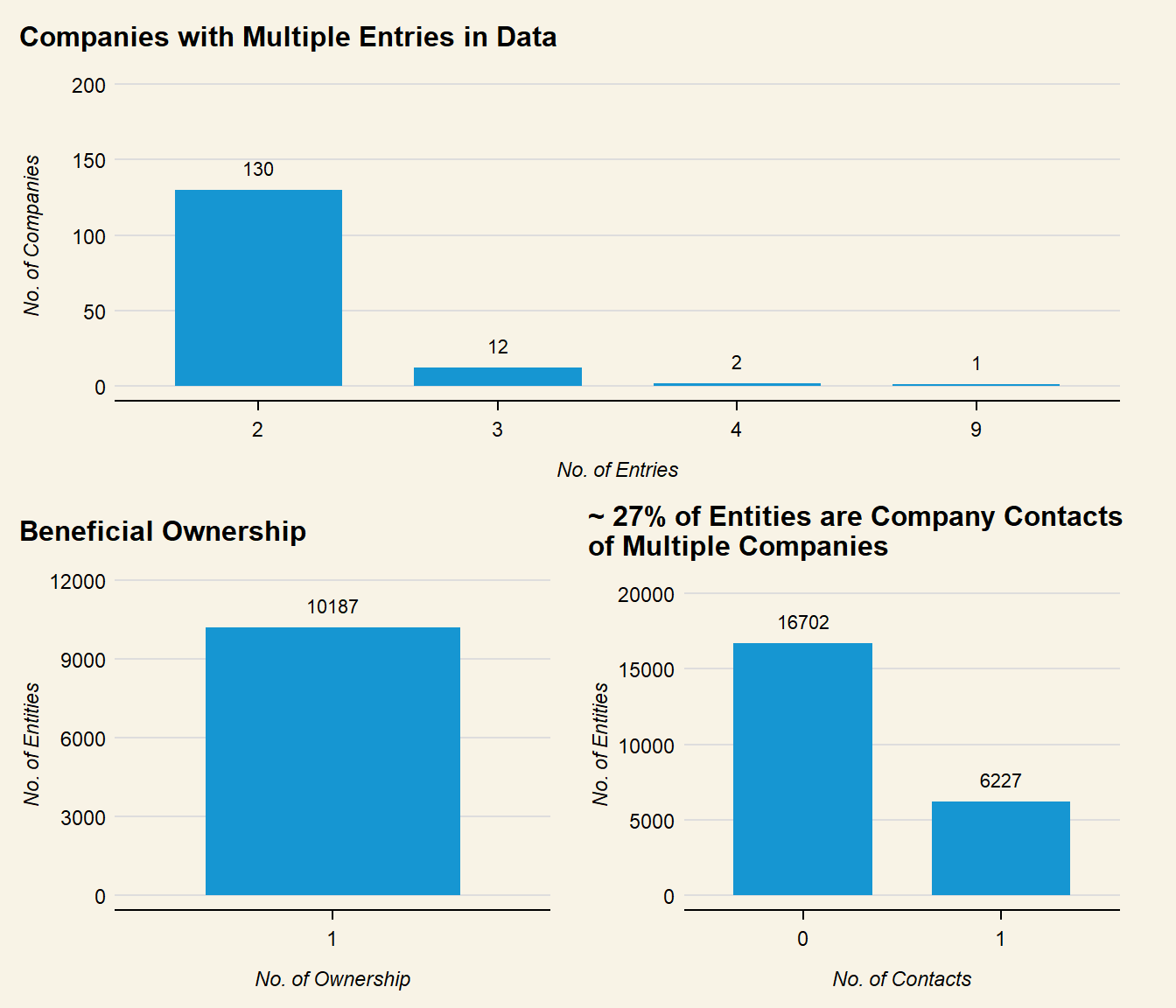
3.1.4: Are there Entities with Multiple Entries?

Similarly to Section 3.1.3, Entities in the Nodes dataframe could possess multiple roles within the network, or operate from different countries. As this may point towards fishy structures, this data is investigated further:

nodes_multiple <- mc3_nodes_new %>%
  group_by(id) %>%
  summarise(count = n()) %>%
  # Only retain entities with multiple roles
  filter(count >1) %>%
  arrange(desc(count)) %>%
  ungroup()

datatable(nodes_multiple)

Data above reveals that there are 1,464 Entities that may have multiple entries. This is investigated further:

code block

nodes_by_type <- mc3_nodes_new %>%
  group_by(id, type) %>%
  summarise(count = n()) %>%
  # Pivot to get each type as a separate column
  pivot_wider(names_from = type, values_from = count, values_fill = 0) %>%
  arrange(desc(Company)) %>%
  ungroup()

company_plot <- nodes_by_type %>%
  # Only get count of nodes with multiple company entries
  filter(Company >1) %>%
  # Show discrete count labels in x axis
  mutate(Company = as.factor(Company)) %>%
  ggplot(
    aes(x = Company)
  ) +
  geom_bar() +
  labs(
    title = "Companies with Multiple Entries in Data",
    x = "No. of Entries",
    y = "No. of Companies"
  ) +
  geom_text(
    stat = "count",
    aes(label = after_stat(count)),
    vjust = -1
  ) +
  ylim(0, 200) +
  theme(
    text = element_text(size = 12),
    plot.background = element_rect(fill="#F8F3E6",colour="#F8F3E6")
  )

owner_plot <- nodes_by_type %>%
  # Only find nodes that are owners
  filter(`Beneficial Owner` >0) %>%
  # Show discrete count labels in x axis
  mutate(`Beneficial Owner` = as.factor(`Beneficial Owner`)) %>%
  ggplot(
    aes(x = `Beneficial Owner`)
  ) +
  geom_bar() +
  labs(
    title = "Beneficial Ownership",
    x = "No. of Ownership",
    y = "No. of Entities"
  ) +
  ylim(0, 11500) +
  geom_text(
    stat = "count",
    aes(label = after_stat(count)),
    vjust = -1
  ) +
  theme(
    text = element_text(size = 12),
    plot.background = element_rect(fill="#F8F3E6",colour="#F8F3E6")
  )

cc_plot <- nodes_by_type %>%
  # Show discrete count labels in x axis
  mutate(`Company Contacts` = as.factor(`Company Contacts`)) %>%
  ggplot(
    aes(x = `Company Contacts`)
  ) +
  geom_bar() +
  labs(
    title = "~ 27% of Entities are Company Contacts\nof Multiple Companies",
    x = "No. of Contacts",
    y = "No. of Entities"
  ) +
  geom_text(
    stat = "count",
    aes(label = after_stat(count)),
    vjust = -1
  ) +
  ylim(0,20000) +
  theme(
    text = element_text(size = 12),
    plot.background = element_rect(fill="#F8F3E6",colour="#F8F3E6")
  )

patch <- owner_plot + cc_plot 
full_patch <- company_plot / patch
full_patch & theme(plot.background = element_rect(fill="#F8F3E6",colour="#F8F3E6"))

Extracting Links from nodes_multiple table

links_multiple <- mc3_links_new %>%
  filter(source %in% nodes_multiple$id) %>%
  rename("from" = "source",
         "to" = "target")

Getting Distinct Source and Target

# Get distinct Source and Target
multiple_source <- links_multiple %>%
  distinct(from) %>%
  rename("id" = "from")

multiple_target <- links_multiple %>%
  distinct(to) %>%
  rename("id" = "to")

Creating Nodes and Edges Dataframes

# Bind into single dataframe
nodes_multiple_new <- bind_rows(multiple_source, multiple_target) %>% distinct()

nodes_multiple_new <- nodes_multiple_new %>%
  left_join(nodes_multiple, by = "id") %>%
  rename("value" = "count") %>%
  # Assign value to number of entries each company has in dataframe
  mutate(value = ifelse(is.na(value), 1, value*5)) %>%
  select(id, value)
  

cc_nodes <- mc3_links_new %>%
  filter(type == "Company Contacts")

nodes_multiple_new$group <- ifelse(nodes_multiple_new$id %in% company_nodes$id, "Company",
                              ifelse(nodes_multiple_new$id %in% cc_nodes$target, "Company Contacts", "Beneficial Owner" ))

code block

visNetwork(
    nodes_multiple_new, 
    links_multiple,
    width = "100%",
    main = list(text = "Variety of Company Structures",
                style = "font-size:17x;
                weight:bold;
                text-align:right;")
  ) %>%
  visIgraphLayout(
    layout = "layout_with_fr"
  ) %>%
  visGroups(groupname = "Company",
            color = "#1696d2") %>%
  visGroups(groupname = "Beneficial Owner",
            color = "#fccb41") %>%
  visGroups(groupname = "Company Contacts",
            color = "#eb99c2") %>%
  visLegend() %>%
  visEdges() %>%
  visOptions(
  # Specify additional Interactive Elements
    highlightNearest = list(enabled = T, degree = 2, hover = T),
  # Add drop-down menu to filter by company name
    nodesIdSelection = TRUE,
  # Add drop-down menu to filter by category
    selectedBy = "group",
    collapse = TRUE) %>%
  visInteraction(navigationButtons = TRUE)

Insights from Visualisations:

Node size is pegged to number of entries per company in the dataframe. As the size of the company node does not seem proportional to number of links (type), this suggests that the multiple entries are due to the company operating across different countries instead.

3.1.5: What Companies are operating across country borders?

The fishing industry is a transboundary operation, and vessels or companies that operate between different jurisdictions may often evade law enforcement authorities. Entities with multiple entries and listed countries could be related to fishy networks. These are filtered and visualised:

Extracting Nodes and Links from companies operating across countries

# Create a filter dataframe to get companies operating across 3 countries
nodes_companies <- nodes_by_type %>%
  filter(Company >= 3)

trans_nodes <- mc3_nodes_new %>%
  filter(id %in% nodes_companies$id)

trans_links <- mc3_links_new %>%
  filter(source %in% trans_nodes$id) %>%
  rename("from" = "source",
         "to" = "target")

Getting Distinct Source and Target

# Get distinct Source and Target
trans_source <- trans_links %>%
  distinct(from) %>%
  rename("id" = "from")

trans_target <- trans_links %>%
  distinct(to) %>%
  rename("id" = "to")

Creating Nodes and Edges Dataframes

# Bind into single dataframe
trans_nodes_new <- bind_rows(trans_source, trans_target) %>% distinct()

# Get country count for each company node
trans_nodes_new <- trans_nodes_new %>%
  left_join(nodes_companies, by= "id") %>%
  rename("value" = "Company") %>%
# Assign value to number of countries each company is operating in
  mutate(value = ifelse(is.na(value), 1, value*5)) %>%
  select(id, value)

trans_nodes_new$group <- ifelse(trans_nodes_new$id %in% company_nodes$id, "Company",
                              ifelse(trans_nodes_new$id %in% cc_nodes$target, "Company Contacts", "Beneficial Owner" ))

code block

visNetwork(
    trans_nodes_new, 
    trans_links,
    width = "100%",
    main = list(text = "Companies Operating Across Borders",
                style = "font-size:17x;
                weight:bold;
                text-align:right;"),
    submain = list(text = "Node size represents Country Count",
                style = "font-size:12x;
                text-align:right;")
  ) %>%
  visIgraphLayout(
    layout = "layout_with_fr"
  ) %>%
  visGroups(groupname = "Company",
            color = "#1696d2") %>%
  visGroups(groupname = "Beneficial Owner",
            color = "#fccb41") %>%
  visGroups(groupname = "Company Contacts",
            color = "#eb99c2") %>%
  visLegend() %>%
  visEdges() %>%
  visOptions(
  # Specify additional Interactive Elements
    highlightNearest = list(enabled = T, degree = 2, hover = T),
  # Add drop-down menu to filter by company name
    nodesIdSelection = TRUE,
  # Add drop-down menu to filter by category
    selectedBy = "group",
    collapse = TRUE) %>%
  visInteraction(navigationButtons = TRUE)

3.2: What are the most common products/services?

%%{
  init: {
    "theme": "base",
    "themeVariables": {
      "primaryColor": "#d8e8e6",
      "primaryTextColor": "#325985",
      "primaryBorderColor": "#325985",
      "lineColor": "#325985",
      "secondaryColor": "#cedded",
      "tertiaryColor": "#fff" 
      }
  }
}%%

flowchart LR
    A{Overall\nNetwork} --> B{Fishy\nCompanies}
    B --> C(Business Type) -.->|Dubious?|D[Products or\nServices]

3.2.1: Data Preparation: Tokenisation

#|code-fold: true
# Replace all 'character(0)' values as unknown
mc3_nodes_new$product_services[mc3_nodes_new$product_services == "character(0)"] <- "Unknown"

# Create new dataframe with words split into separate rows
nodes_unnest <- mc3_nodes_new %>%
  # Create new column 'word' to store split words
  unnest_tokens(word, 
                product_services,
    # Change all words to lowercase for more accurate tokenisation
                to_lower = TRUE,
    # Remove punctuation to exclude from tokenisation
                strip_punct = TRUE)

# Create a vector containing only the text
nodes_text <- nodes_unnest$word 

# Create a corpus
text <- Corpus(VectorSource(nodes_text))

The process of removing specific stopwords using removeWords is an iterative process, where higher frequency words are removed if deemed out of context (such as ‘well’, ‘including’, ‘related’ or unproductive in giving specific information about the nature of businesses (such as ‘source’, ‘materials’, etc).

text <- text %>%
  # Remove any whitespace
  tm_map(stripWhitespace) %>%
  # remove stopwords
  tm_map(removeWords, stopwords(kind = "en")) %>%
  # Specity stopwords based on initial analysis of word frequency
  tm_map(removeWords, c("products", "including", "well", "related", "services", "source", "materials", "goods", "offers", "range"))

# Generate a document-term-matrix
dtm <- TermDocumentMatrix(text) 
matrix <- as.matrix(dtm) 
# Sort matrix according to frequency
words <- sort(rowSums(matrix),decreasing = TRUE) 
# Count frequency of each word and save as new column in dataframe
text_df <- data.frame(word = names(words),freq = words)

kable(head(text_df,15))

	word	freq
unknown	unknown	21004
fish	fish	740
seafood	seafood	622
frozen	frozen	467
food	food	345
equipment	equipment	309
fresh	fresh	276
salmon	salmon	252
accessories	accessories	193
systems	systems	180
freight	freight	176
industrial	industrial	164
canned	canned	163
meat	meat	157
processing	processing	155

The table output shows that “Unknown” products and services are the most frequently listed. While this could possibly point to fishy business relationships, these records may also be masking other anomalies present. A separate text dataframe is created without “unknown” products and services:

text_df_known <- text_df[-1,]

code block

wordcloud2(text_df_known, 
           color = "random-dark", 
           backgroundColor = "#F8F3E6")

3.2.2: Plotting a Bigram of frequent Products/Services

nodes_unnest2 <- mc3_nodes %>%
   unnest_tokens(bigram, 
                 product_services, 
                 token = "ngrams", 
                 n = 2, 
                 to_lower = TRUE,) %>%
  # remove empty rows
   filter(!is.na(bigram)) %>%
  # Remove specific stopwords from bigrams
   filter(!str_detect(bigram,"including|range|related|freelance"))

product_bigram <- nodes_unnest2 %>%
    count(bigram, sort = TRUE) %>%
  # Split bigram words into separate columns, uding space as delimiter
    separate(bigram, c("word1", "word2"), sep = " ") %>%
  # Only match words not in stopwords
    anti_join(stop_words, by = c("word1" = "word")) %>%
    anti_join(stop_words, by = c("word2" = "word")) %>%
  # Keep only characters, dropping numbers 
    filter(str_detect(word1, "[a-z]") & str_detect(word2, "[a-z]"))

Applying a filter to keep only most frequently related bigrams

product_bigram_graph <- product_bigram %>%
  filter(n >15) %>%
  graph_from_data_frame()

code block

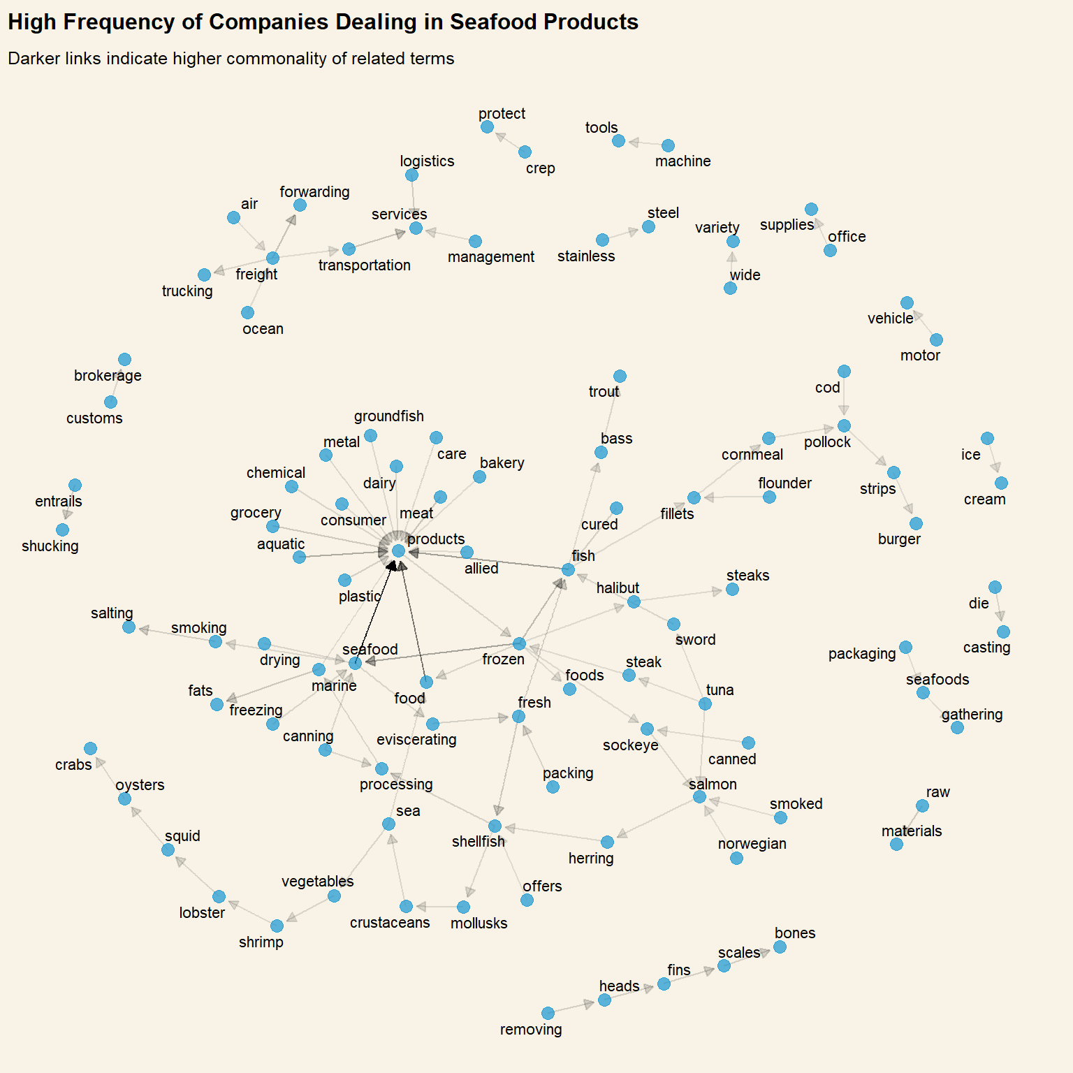
set.seed(1234)
ggraph(
  product_bigram_graph, 
  layout = "nicely"
  ) +
  geom_edge_link(
    # Adjust transparency of link based on how common the bigram is
    aes(edge_alpha = n),
    arrow = grid::arrow(type = "closed", 
                        length = unit(.2, "cm")),
    # Leave a gap between arrow head and circle
    end_cap = circle(.2, 'cm'),
    show.legend = FALSE
  ) +
  geom_node_point(
    alpha = .7,
    size = 3) +
  geom_node_text(
    aes(label = name), 
    repel = TRUE
  ) +
  labs(title = "High Frequency of Companies Dealing in Seafood Products",
       subtitle = "Darker links indicate higher commonality of related terms"
  ) +
  theme(plot.background = element_rect(fill="#F8F3E6",colour="#F8F3E6")
  )

code block

datatable(product_bigram)

Insights from Visualisations:

Explorations revealed that most frequently declared products/services are related to the fishing industry. This is unsurprising.
A high number of other food-related and shipping-related services were also uncovered. In fact, companies that provide non fishing-related products or services could be filtered out as possible brokers for fishy networks
There are several overlaps in the frequent bigrams, that may be grouped together as the same category. The most frequent bigrams and words in the wordcloud above will be used as a base for product/service company categories.

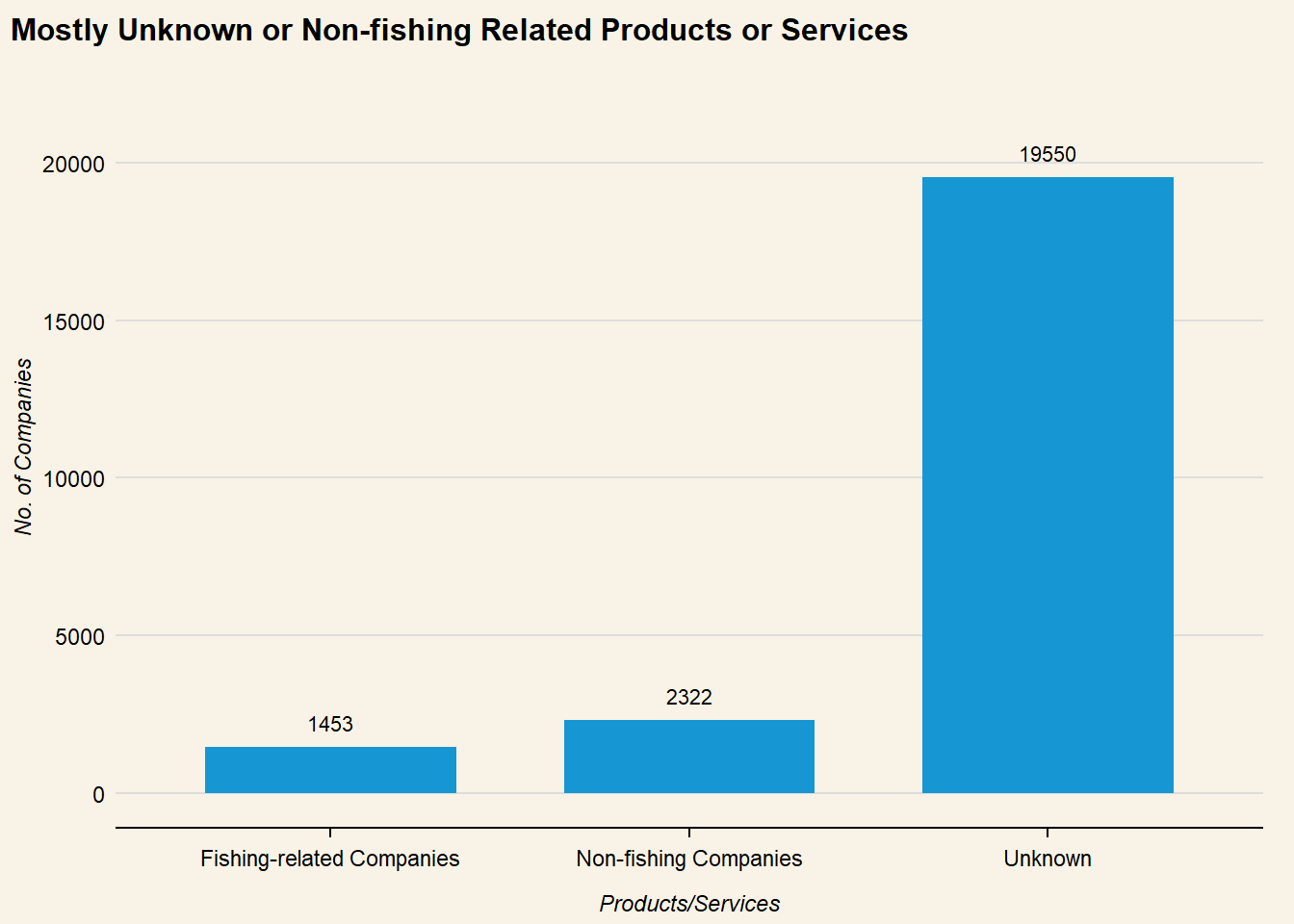
3.3: Can the Companies be grouped according to Products/Services provided?

The text analysis in section 3.2 was used to deduce categories for products and services. As non-fishing or non-food related companies within the network could be masking fishy company structures, the nodes are categorised as:

Products/Services	Inclusive of:
Fishing-related Companies	fish products, food products, food processing, marine products
Non-fishing Companies	freight forwarding, transportation services, logistics services, equipment, machinery, etc
Unknown	Unknown

code block

# Create nodes dataframe with unique node ids
mc3_nodes_agg <- mc3_nodes_new %>%
  group_by(id, type,) %>%
  summarise(count = n(),
            product_services = paste(product_services, collapse = ", ")) %>%
  # Pivot to get each type as a separate column
  pivot_wider(names_from = type, values_from = count, values_fill = 0) %>%
  ungroup()

`summarise()` has grouped output by 'id'. You can override using the `.groups`
argument.

code block

mc3_nodes_cat <- mc3_nodes_agg

mc3_nodes_cat$prod_group <- 
  ifelse(grepl("fish|frozen|shellfish|fresh fish|seafood|food|meat|
               dairy|vegetable|grocery|entrails|shucking|smoking|salting|
               processing|packaging|canning|packing|aquatic products|
               marine fats|fins|scales|tuna", 
          mc3_nodes_agg$product_services, ignore.case = TRUE), "Fishing-related Companies",
  ifelse(grepl("unknown",
        mc3_nodes_agg$product_services, ignore.case = TRUE), "Unknown", "Non-fishing Companies"))

nodes_cat_plot <- mc3_nodes_cat %>%
  mutate(prod_group = as.factor(prod_group)) %>%
  ggplot(
    aes(x = prod_group)
  ) +
  geom_bar() +
  labs(
    title = "Mostly Unknown or Non-fishing Related Products or Services",
    x = "Products/Services",
    y = "No. of Companies"
  ) +
  geom_text(
    stat = "count",
    aes(label = after_stat(count)),
    vjust = -1
  ) +
  ylim(0, 22000) +
  theme(
    text = element_text(size = 12),
    plot.background = element_rect(fill="#F8F3E6",colour="#F8F3E6")
  )

nodes_cat_plot

4: A Fishy Network

Exploratory analysis thus far has revealed some underlying structures of various groups within the network. The most anomalous (and interlinked) sub-networks, High Revenue and High Link Count and Beneficial Owners with Multiple Companies, are concatenated to further investigate if these fishy structures are interlinked, as well as grouping companies and entities by categories.

The “group” that the entity is assigned is based on the following roles:

Group	Logic
Ultimate Beneficial Owner	Beneficial Owner of >= 20 Companies, a key player in the network
Multi-role Entity	Plays multiple roles within the network, may be a key personnel or broker within the network
Beneficial Owner	Shareholder of the company
Companies	May be Fishing-related, Non-fishing related or offering Unknown products/services

Creating Nodes and Links Dataframes

links_owner and links_highrev are merged

links_merged <- bind_rows(links_owner, links_highrev) %>% distinct()

merged_source <- links_merged %>%
  distinct(from) %>%
  rename("id" = "from")

merged_target <- links_merged %>%
  distinct(to) %>%
  rename("id" = "to")

nodes_merged <- bind_rows(merged_source, merged_target) %>% distinct()

Updating Nodes Groups

# Create a separate column counting no of different roles each entity takes on
mc3_nodes_cat$cat_count <- rowSums(mc3_nodes_cat[, c("Company", "Beneficial Owner", "Company Contacts")] >0)

nodes_merged_new <- nodes_merged %>%
  # Get product category info
  left_join(mc3_nodes_cat, by = "id") %>%
  select(id, prod_group, cat_count) %>%
  rename("type" = "prod_group") %>%
  
  # Get number of linked companies per beneficial owner/company contact
  left_join(links_by_target, by= join_by("id" == "target")) %>%
  # merge values from type column
  mutate(type = coalesce(type.x, type.y)) %>%
  select(id, type, company_count, cat_count) %>%
  
  # rename variables for visNetwork
  rename("value" = "company_count") %>%
  
  # Assign values to nodes as size in visNetwork
  mutate(value = ifelse(is.na(value), 1, value*5)) %>%
  rename("group" = "type") %>%
  select(id, group, value, cat_count) %>%
  distinct()

Assigning Group Logic to nodes

# Assigning Ultimate Beneficial Owner status
nodes_merged_new$group <- ifelse(nodes_merged_new$value >= 20 & nodes_merged_new$group == "Beneficial Owner",
                               yes = "Ultimate Beneficial Owner",
                              # Remain as is
                               no = nodes_merged_new$group)

# Create filter from original links and nodes dataframe
links_combined_cc <- mc3_links_new %>%
  filter(type == "Company Contacts") %>%
  select(target, type) %>%
  rename("id" = "target")

nodes_cc <- mc3_nodes_new %>%
  filter(type == "Company Contacts") %>%
  select(id, type) %>%
  bind_rows(links_combined_cc) %>%
  select(id, type) %>%
  distinct()

links_combined_bo <- mc3_links_new %>%
  filter(type == "Beneficial Owner") %>%
  select(target, type) %>%
  rename("id" = "target")

nodes_bo <- mc3_nodes_new %>%
  filter(type == "Beneficial Owner") %>%
  select(id, type) %>%
  bind_rows(links_combined_bo) %>%
  select(id, type) %>%
  distinct()

# Replace NA values in column based on conditional values
nodes_merged_new$group <- ifelse(is.na(nodes_merged_new$group),
                             ifelse(nodes_merged_new$id %in% nodes_cc$id, "Company Contacts", "?"),
                             nodes_merged_new$group)

nodes_merged_new$group <- ifelse((nodes_merged_new$group == "?"),
                             ifelse(nodes_merged_new$id %in% nodes_bo$id, "Beneficial Owner", "Unknown"),
                             nodes_merged_new$group)  

nodes_merged_new <- nodes_merged_new %>%
  mutate(value = ifelse(is.na(value), 1, value)) %>%
  select(id, group, value)

Filtering out nodes with multiple roles

# Create filter based on nodes with multiple roles
nodes_merged_filter <- nodes_merged_new %>%
  group_by(id) %>%
  summarise(value = sum(value),
            count = n()) %>%
  ungroup() %>%
  filter(count >1)

# remove nodes from nodes_merged_new dataframe
nodes_merged_new <- nodes_merged_new %>%
  filter(!(id %in% nodes_merged_filter$id))

# Assign group to nodes with multiple roles
nodes_merged_filter <- nodes_merged_filter %>%
  mutate(group = "Multi-role Entity") %>%
  select(id, group, value)

# Append back to nodes dataframe
nodes_merged_new <- bind_rows(nodes_merged_new, nodes_merged_filter)

code block

visNetwork(
    nodes_merged_new, 
    links_merged,
    width = "100%"
  ) %>%
  visIgraphLayout(
    layout = "layout_with_fr"
  ) %>%
  visGroups(groupname = "Ultimate Beneficial Owner", 
            shape = "icon",
            icon = list(code = "f521",
                        size = 80,
                        color = "#e25552")) %>%
  visGroups(groupname = "Beneficial Owner",
            shape = "icon",
            icon = list(code = "f2bd",
                        size = 45,
                        color = "#fccb41")) %>%
  visGroups(groupname = "Multi-role Entity",
            shape = "icon",
            icon = list(code = "f21b",
                        color = "#695790")) %>%
  visGroups(groupname = "Fishing-related Companies",
            shape = "icon",
            icon = list(code = "f21a",
                        color = "#1696d2")) %>%
  visGroups(groupname = "Non-fishing Companies",
            shape = "icon",
            icon = list(code = "f0b1",
                        color = "#6CC3A5")) %>%
  visGroups(groupname = "Unknown",
            shape = "icon",
            icon = list(code = "f059",
                        color = "#5c5859")) %>%
  visLegend() %>%
  visEdges() %>%
  addFontAwesome() %>%
  visOptions(
  # Specify additional Interactive Elements
    highlightNearest = list(enabled = T, degree = 2, hover = T),
  # Add drop-down menu to filter by company name
    nodesIdSelection = TRUE,
  # Add drop-down menu to filter by category
    selectedBy = "group",
    collapse = TRUE) %>%
  visInteraction(navigationButtons = TRUE)

The Various structures of the companies in the Network Graph with the roles of entities assigned can be summarised in the following flowchart:

%%{
  init: {
    "theme": "base",
    "themeVariables": {
      "primaryColor": "#d8e8e6",
      "primaryTextColor": "#325985",
      "primaryBorderColor": "#325985",
      "lineColor": "#325985",
      "secondaryColor": "#cedded",
      "tertiaryColor": "#fff" 
      }
  }
}%%

flowchart LR
    A{Overall\nNetwork} --> B{Fishy\nCompany\nStructures}
    B --> C(fa:fa-star-of-life\nShell/Front\nCompany) -.-|Two or More|D(Companies)
    C -.-|Overlapping|E(fa:fa-users Beneficial Owners)
    C -.-|+ Multi-role Entity|F(fa:fa-user-secret Broker)
    B --> G(fa:fa-link\nJoint Venture) -.-|Multiple|H(fa:fa-diagram-project Company Networks)
    G -.-|linked by|I(fa:fa-users Beneficial Owners)
    G -.-|Multiple|J(Company Types)
    B --> K(fa:fa-arrows-to-dot\nSole\nProprietorship) -.-|Several|L(Companies)
    K -.-|Single|M(fa:fa-circle-user Beneficial Owner)
    B --> N(fa:fa-building\nPublicly-listed\nCompany) -.-|Numerous|O(fa:fa-users Beneficial Owners)
    N -.-|Single|P(Company)