Hands on Exercise 4

Load and Install R Packages

pacman::p_load(ggstatsplot, tidyverse)

Importing the data

exam_data <- read_csv("data/Exam_data.csv")

head(exam_data, 10)

# A tibble: 10 × 7
   ID         CLASS GENDER RACE    ENGLISH MATHS SCIENCE
   <chr>      <chr> <chr>  <chr>     <dbl> <dbl>   <dbl>
 1 Student321 3I    Male   Malay        21     9      15
 2 Student305 3I    Female Malay        24    22      16
 3 Student289 3H    Male   Chinese      26    16      16
 4 Student227 3F    Male   Chinese      27    77      31
 5 Student318 3I    Male   Malay        27    11      25
 6 Student306 3I    Female Malay        31    16      16
 7 Student313 3I    Male   Chinese      31    21      25
 8 Student316 3I    Male   Malay        31    18      27
 9 Student312 3I    Male   Malay        33    19      15
10 Student297 3H    Male   Indian       34    49      37

One-Sample Test: gghistostats()

set.seed(1234)

gghistostats(
  data = exam_data,
  x = ENGLISH,
  type = "bayes",
  test.value = 60,
  xlab = "English scores") + 
  theme_classic() +
  theme(plot.background = element_rect(fill = "#F8F3E6", color = "#F8F3E6"))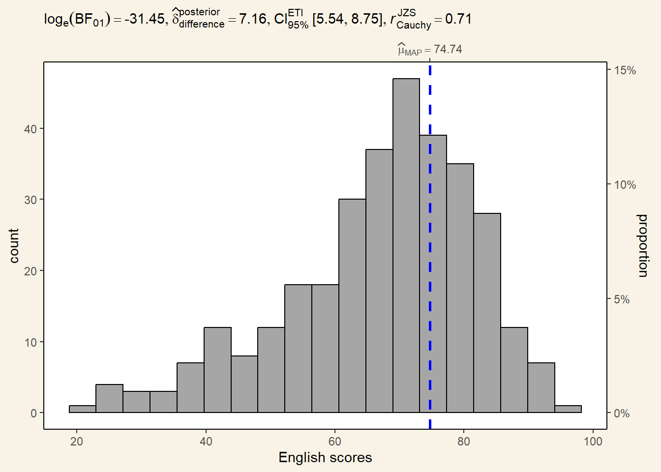

Bayes factor is the ratio of the likelihood of one particular hypothesis to the likelihood of another. It can be interpreted as a measure of the strength of evidence in favor of one theory among two competing theories.

Two-Sample Test of difference in means: ggbetweenstats()

ggbetweenstats(
  data = exam_data,
  x = GENDER, 
  y = MATHS,
  type = "np",
  messages = FALSE) +
  theme_classic() +
  theme(plot.background = element_rect(fill = "#F8F3E6", color = "#F8F3E6"))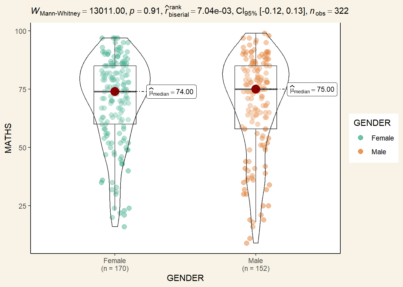

One-way ANOVA Test of difference in means: ggbetweenstats()

ggbetweenstats(
  data = exam_data,
  x = RACE, 
  y = ENGLISH,
  type = "p",
  mean.ci = TRUE, 
  pairwise.comparisons = TRUE, 
  pairwise.display = "s",
  p.adjust.method = "fdr",
  messages = FALSE) +
  theme_classic() +
  theme(plot.background = element_rect(fill = "#F8F3E6", color = "#F8F3E6"))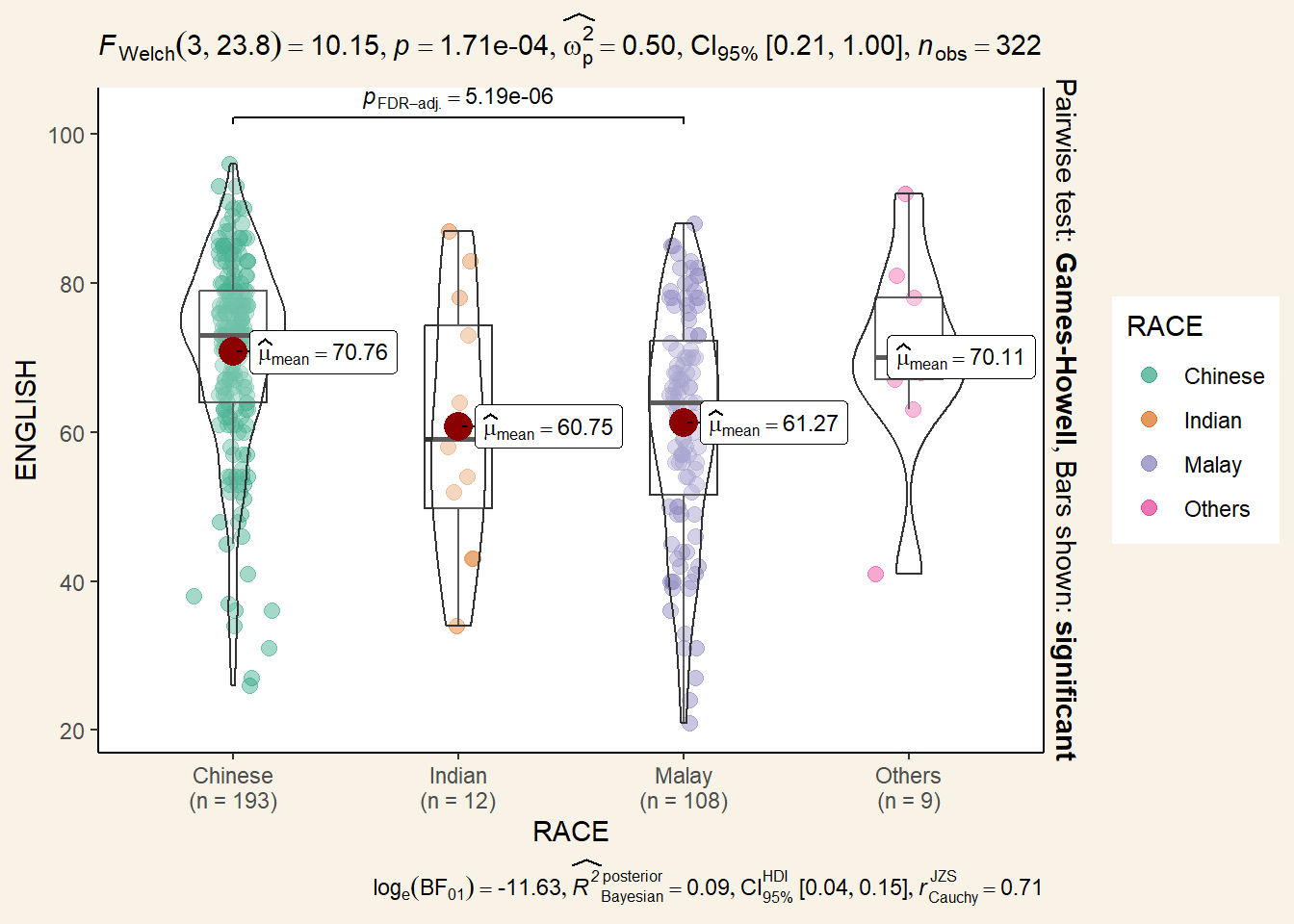

Correlation Test: ggscatterstats()

ggscatterstats(
  data = exam_data,
  x = MATHS,
  y = ENGLISH,
  marginal = FALSE) +
  theme_classic() +
  theme(plot.background = element_rect(fill = "#F8F3E6", color = "#F8F3E6"))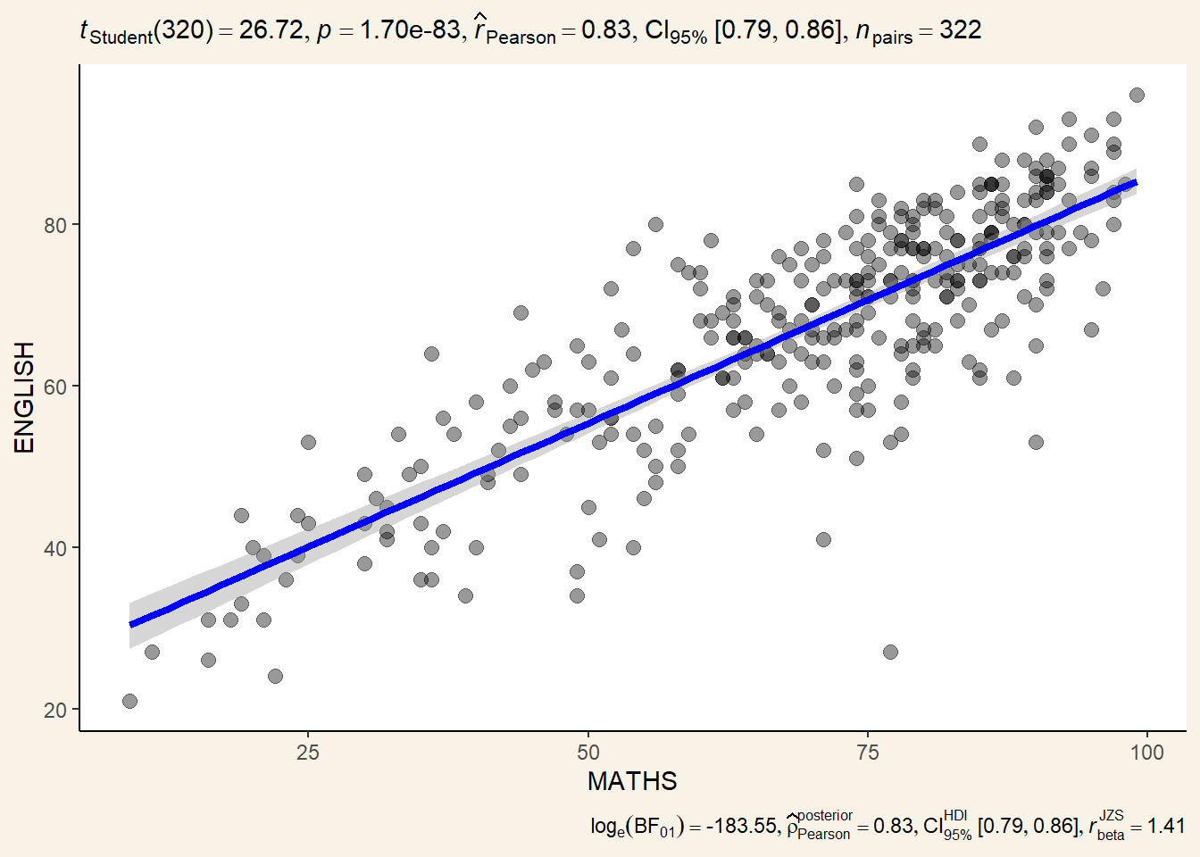

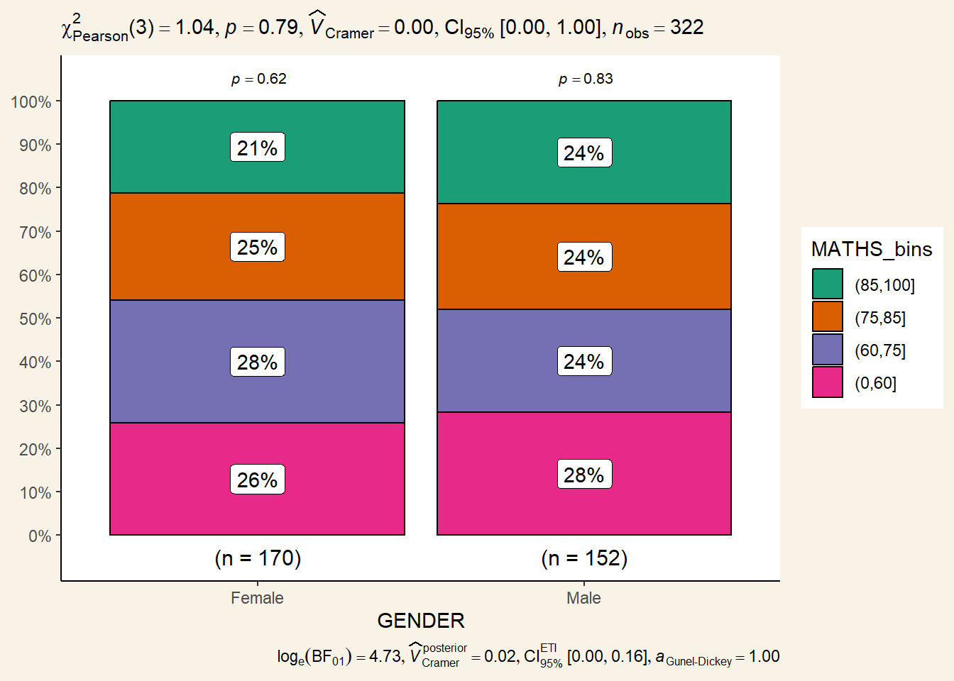
Association Test (Dependence): ggbarstats()

exam1 <- exam_data %>% 
  mutate(MATHS_bins = 
           cut(MATHS, 
               breaks = c(0,60,75,85,100))
)

ggbarstats(exam1, 
           x = MATHS_bins, 
           y = GENDER) +
  theme_classic() +
  theme(plot.background = element_rect(fill = "#F8F3E6", color = "#F8F3E6"))